Hypothesis testing is one of the most widely used approaches of statistical inference.
The idea of hypothesis testing (more formally: null hypothesis significance testing - NHST) is the following: if we have some data observed, and we have a statistical model, we can use this statistical model to specify a fixed hypothesis about how the data did arise. For the example with the plants and music, this hypothesis could be: music has no influence on plants, all differences we see are due to random variation between individuals.
The null hypothesis H0 and the alternative hypothesis H1
Such a scenario is called the null hypothesis H0. Although it is very typical to use the assumption of no effect as null-hypothesis, note that it is really your choice, and you could use anything as null hypothesis, also the assumption: “classical music doubles the growth of plants”. The fact that it’s the analyst’s choice what to fix as null hypothesis is part of the reason why there are are a large number of tests available. We will see a few of them in the following chapter about important hypothesis tests.
The hypothesis that H0 is wrong, or !H0, is usually called the alternative hypothesis, H1
Given a statistical model, a “normal” or “simple” null hypothesis specifies a single value for the parameter of interest as the “base expectation”. A composite null hypothesis specifies a range of values for the parameter.
p-value
If we have a null hypothesis, we calculate the probability that we would see the observed data or data more extreme under this scenario. This is called a hypothesis tests, and we call the probability the p-value. If the p-value falls under a certain level (the significance level $\alpha$) we say the null hypothesis was rejected, and there is significant support for the alternative hypothesis. The level of $\alpha$ is a convention, in ecology we chose typically 0.05, so if a p-value falls below 0.05, we can reject the null hypothesis.
Test Statistic
Type I and II error
Significance level, Power
Misinterpretations
A problem with hypothesis tests and p-values is that their results are notoriously misinterpreted. The p-value is NOT the probability that the null hypothesis is true, or the probability that the alternative hypothesis is false, although many authors have made the mistake of interpreting it like that \citep[][]{Cohen-earthisround-1994}. Rather, the idea of p-values is to control the rate of false positives (Type I error). When doing hypothesis tests on random data, with an $\alpha$ level of 0.05, one will get exactly 5\% false positives. Not more and not less.
Further readings
- The Essential Statistics lecture notes
- http://www.stats.gla.ac.uk/steps/glossary/hypothesis_testing.html
Examples in R
Recall statistical tests, or more formally, null-hypothesis significance testing (NHST) is one of several ways in which you can approach data. The idea is that you define a null-hypothesis, and then you look a the probability that the data would occur under the assumption that the null hypothesis is true.
Now, there can be many null hypothesis, so you need many tests. The most widely used tests are given here.
library(knitr)
opts_knit$set(global.par=TRUE)
opts_chunk$set(cache.extra = rand_seed,fig.align='center')
set.seed(12)
t-test
The t-test can be used to test whether one sample is different from a reference value (e.g. 0: one-sample t-test), whether two samples are different (two-sample t-test) or whether two paired samples are different (paired t-test).
The t-test assumes that the data are normally distributed. It can handle samples with same or different variances, but needs to be “told” so.
t-test for 1 sample (PARAMETRIC TEST)
The one-sample t-test compares the MEAN score of a sample to a known value, usually the population MEAN (the average for the outcome of some population of interest).
data = read.table("../Data/Simone/das.txt",header=T)
attach(data)
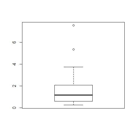
boxplot(y)

Our null hypothesis is that the mean of the sample is not less than 2.5 (real example: weight data of 200 lizards collected for a research, we want to compare it with the known average weights available in the scientific literature)
t.test(y,mu=2.5,alt="less",conf=0.95) # mean = 2.5, alternative hypothesis one-sided; we get a one-sided 95% CI for the mean
##
## 	One Sample t-test
##
## data:  y
## t = -3.3349, df = 99, p-value = 0.000601
## alternative hypothesis: true mean is less than 2.5
## 95 percent confidence interval:
##      -Inf 2.459557
## sample estimates:
## mean of x
##  2.419456
t.test(y,mu=2.5,alt="two.sided",conf=0.95) #2 sided-version
##
## 	One Sample t-test
##
## data:  y
## t = -3.3349, df = 99, p-value = 0.001202
## alternative hypothesis: true mean is not equal to 2.5
## 95 percent confidence interval:
##  2.371533 2.467379
## sample estimates:
## mean of x
##  2.419456
detach(data)
t-test for 1 sample (NON-PARAMETRIC TEST)
One-sample Wilcoxon signed rank test is a non-parametric alternative method of one-sample t-test, which is used to test whether the location (MEDIAN) of the measurement is equal to a specified value
Create fake data log-normally distributed and verify data distribution
x<-exp(rnorm(15))
plot(x)

boxplot(x)

qqnorm(x)
qqline(x,lty=2,col=2,lwd=3)
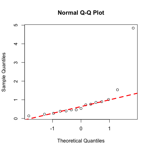
shapiro.test(x) # not normally distributed
##
## 	Shapiro-Wilk normality test
##
## data:  x
## W = 0.5674, p-value = 1.297e-05
summary(x)
##    Min. 1st Qu.  Median    Mean 3rd Qu.    Max.
##  0.1357  0.3913  0.5335  0.9005  0.8788  4.8410
Our null hypothesis is that the median of x is not different from 1
wilcox.test(x, alternative="two.sided", mu=1) # high p value-> median of x is not different from 1
##
## 	Wilcoxon signed rank test
##
## data:  x
## V = 23, p-value = 0.03534
## alternative hypothesis: true location is not equal to 1
Two Independent Samples T-test (PARAMETRIC TEST)
Parametric method for examining the difference in MEANS between two independent populations. The t-test should be preceeded by a graphical depiction of the data in order to check for normality within groups and for evidence of heteroscedasticity (= differences in variance), like so:
Reshape the data:
Y1 <- rnorm(20)
Y2 <- rlnorm(20)
Y <- c(Y1, Y2)
groups <- as.factor(c(rep("Y1", length(Y1)), rep("Y2", length(Y2))))
Now plot them as points (not box-n-whiskers):
plot.default(Y ~ groups)

The points to the right scatter similar to those on the left, although a bit more asymmetrically. Although we know that they are from a log-normal distribution (right), they don’t look problematic.
If data are not normally distributed, we sometimes succeed making data normal by using transformations, such as square-root, log, or alike (see section on transformations).
While t-tests on transformed data now actually test for differences between these transformed data, that is typically fine. Think of the pH-value, which is only a log-transform of the proton concentration. Do we care whether two treatments are different in pH or in proton concentrations? If so, then we need to choose the right data set. Most likely, we don’t and only choose the log-transform because the data are actually lognormally distributed, not normally.
A non-parametric alternative is the Mann-Whitney-U-test, or, the ANOVA-equivalent, the Kruskal-Wallis test. Both are available in R and explained later, but instead we recommend the following:
Use rank-transformations, which replaces the values by their rank (i.e. the lowest value receives a 1, the second lowest a 2 and so forth). A t-test of rank-transformed data is not the same as the Mann-Whitney-U-test, but it is more sensitive and hence preferable (Ruxton 2006) or at least equivalent (Zimmerman 2012).
t.test(rank(Y) ~ groups)
##
## 	Welch Two Sample t-test
##
## data:  rank(Y) by groups
## t = -3.9252, df = 35.266, p-value = 0.000384
## alternative hypothesis: true difference in means is not equal to 0
## 95 percent confidence interval:
##  -18.811615  -5.988385
## sample estimates:
## mean in group Y1 mean in group Y2
##             14.3             26.7
To use the rank, we need to employ the “formula”-invokation of t.test! In this case, results are the same, indicating that our hunch about acceptable skew and scatter was correct.
(Note that the original t-test is a test for differences between means, while the rank-t-test becomes a test for general differences in values between the two groups, not specifically of the mean.)
Cars example:
head(mtcars)
##                    mpg cyl disp  hp drat    wt  qsec vs am gear carb
## Mazda RX4         21.0   6  160 110 3.90 2.620 16.46  0  1    4    4
## Mazda RX4 Wag     21.0   6  160 110 3.90 2.875 17.02  0  1    4    4
## Datsun 710        22.8   4  108  93 3.85 2.320 18.61  1  1    4    1
## Hornet 4 Drive    21.4   6  258 110 3.08 3.215 19.44  1  0    3    1
## Hornet Sportabout 18.7   8  360 175 3.15 3.440 17.02  0  0    3    2
## Valiant           18.1   6  225 105 2.76 3.460 20.22  1  0    3    1
mtcars$fam=factor(mtcars$am, levels=c(0,1), labels=c("automatic","manual")) #transform "am" into a factor (fam) [Transmission (0 = automatic, 1 = manual)]

attach(mtcars)
head(mtcars)
##                    mpg cyl disp  hp drat    wt  qsec vs am gear carb
## Mazda RX4         21.0   6  160 110 3.90 2.620 16.46  0  1    4    4
## Mazda RX4 Wag     21.0   6  160 110 3.90 2.875 17.02  0  1    4    4
## Datsun 710        22.8   4  108  93 3.85 2.320 18.61  1  1    4    1
## Hornet 4 Drive    21.4   6  258 110 3.08 3.215 19.44  1  0    3    1
## Hornet Sportabout 18.7   8  360 175 3.15 3.440 17.02  0  0    3    2
## Valiant           18.1   6  225 105 2.76 3.460 20.22  1  0    3    1
##                         fam
## Mazda RX4            manual
## Mazda RX4 Wag        manual
## Datsun 710           manual
## Hornet 4 Drive    automatic
## Hornet Sportabout automatic
## Valiant           automatic
summary(mtcars$fam)
## automatic    manual
##        19        13
Test the difference in car consumption depending on the transmission type. Check wherever the 2 ‘independent populations’ are normally distributed
par(mfrow=c(1,2))
qqnorm(mpg[fam=="manual"]);qqline(mpg[fam=="manual"])
qqnorm(mpg[fam=="automatic"]); qqline(mpg[fam=="automatic"])

shapiro.test(mpg[fam=="manual"]) #normal distributed
##
## 	Shapiro-Wilk normality test
##
## data:  mpg[fam == "manual"]
## W = 0.9458, p-value = 0.5363
shapiro.test(mpg[fam=="automatic"]) #normal distributed
##
## 	Shapiro-Wilk normality test
##
## data:  mpg[fam == "automatic"]
## W = 0.9768, p-value = 0.8987
par(mfrow=c(1,1))
Graphic representation
boxplot(mpg~fam, ylab="Miles/gallon",xlab="Transmission",las=1)

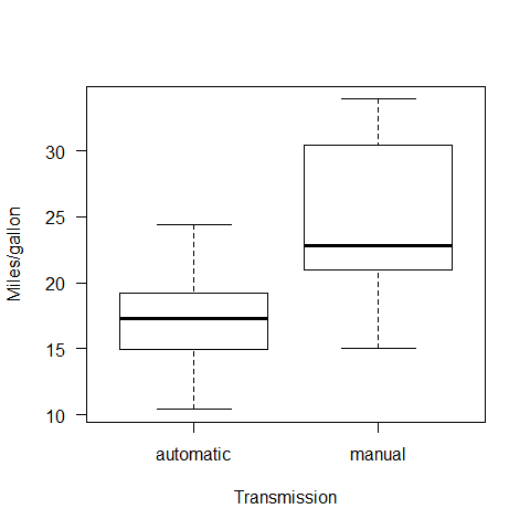
We have two ~normally distributed populations. In order to test for differences in means, we applied a t-test for independent samples.
Any time we work with the t-test, we have to verify whether the variance is equal betwenn the 2 populations or not, then we fit the t-test accordingly.
Our Ho or null hypothesis is that the consumption is the same irrespective to transmission. We assume non-equal variances
t.test(mpg~fam,mu=0, alt="two.sided",conf=0.95,var.eq=F,paired=F)
##
## 	Welch Two Sample t-test
##
## data:  mpg by fam
## t = -3.7671, df = 18.332, p-value = 0.001374
## alternative hypothesis: true difference in means is not equal to 0
## 95 percent confidence interval:
##  -11.280194  -3.209684
## sample estimates:
## mean in group automatic    mean in group manual
##                17.14737                24.39231
From the output: please note that CIs are the confidence intervales for differences in means
Same results if you run the following (meaning that the other commands were all by default)
t.test(mpg~fam)
##
## 	Welch Two Sample t-test
##
## data:  mpg by fam
## t = -3.7671, df = 18.332, p-value = 0.001374
## alternative hypothesis: true difference in means is not equal to 0
## 95 percent confidence interval:
##  -11.280194  -3.209684
## sample estimates:
## mean in group automatic    mean in group manual
##                17.14737                24.39231
The alternative could be one-sided (greater, lesser) as we discussed earlier for one-sample t-tests
If we assume equal variance, we run the following
t.test(mpg~fam,var.eq=TRUE,paired=F)
##
## 	Two Sample t-test
##
## data:  mpg by fam
## t = -4.1061, df = 30, p-value = 0.000285
## alternative hypothesis: true difference in means is not equal to 0
## 95 percent confidence interval:
##  -10.84837  -3.64151
## sample estimates:
## mean in group automatic    mean in group manual
##                17.14737                24.39231
Ways to check for equal / not equal variance
1) To examine the boxplot visually
boxplot(mpg~fam, ylab="Miles/gallon",xlab="Transmission",las=1)

2) To compute the actual variance
var(mpg[fam=="manual"])
## [1] 38.02577
var(mpg[fam=="automatic"])
## [1] 14.6993
There is 2/3 times difference in variance.
3) Levene’s test
library(car)
leveneTest(mpg~fam) # Ho is that the population variances are equal
## Levene's Test for Homogeneity of Variance (center = median)
##       Df F value  Pr(>F)
## group  1  4.1876 0.04957 *
##       30
## ---
## Signif. codes:  0 '***' 0.001 '**' 0.01 '*' 0.05 '.' 0.1 ' ' 1
# Ho rejected, non-equal variances
Mann-Whitney U test/Wilcoxon rank-sum test for two independent samples (NON-PARAMETRIC TEST)
We change the response variable to hp (Gross horsepower)
qqnorm(hp[fam=="manual"]);qqline(hp[fam=="manual"])

qqnorm(hp[fam=="automatic"]);qqline(hp[fam=="automatic"])

shapiro.test(hp[fam=="manual"]) #not normally distributed
##
## 	Shapiro-Wilk normality test
##
## data:  hp[fam == "manual"]
## W = 0.7676, p-value = 0.00288
shapiro.test(hp[fam=="automatic"]) #normally distributed
##
## 	Shapiro-Wilk normality test
##
## data:  hp[fam == "automatic"]
## W = 0.9583, p-value = 0.5403
The ‘population’ of cars with manual transmission has a hp not normally distributed, so we have to use a test for independent samples - non-parametric
We want to test a difference in hp depending on the transmission Using a non-parametric test, we test for differences in MEDIANS between 2 independent populations
boxplot(hp~fam)

Our null hypothesis will be that the medians are equal (two-sided)
wilcox.test(hp~fam,mu=0,alt="two.sided",conf.int=T,conf.level=0.95,paired=F,exact=F) ## non parametric conf.int are reported
##
## 	Wilcoxon rank sum test with continuity correction
##
## data:  hp by fam
## W = 176, p-value = 0.0457
## alternative hypothesis: true location shift is not equal to 0
## 95 percent confidence interval:
##  8.624237e-05 9.199995e+01
## sample estimates:
## difference in location
##               55.00007
detach(mtcars)
Wilcoxon signed rank test for two dependend samples (NON PARAMETRIC)
This is a non-parametric method appropriate for examining the median difference in 2 populations observations that are paired or dependent one of the other.
This is a dataset about some water measurements taken at different levels of a river: ‘up’ and ‘down’ are water quality measurements of the same river taken before and after a water treatment filter, respectively
streams = read.table("../Data/Simone/streams.txt",header=T)
head(streams)
##   down up
## 1   20 23
## 2   15 16
## 3    6 10
## 4    5  4
## 5   20 22
## 6   15 15
attach(streams)
summary(streams)
##       down             up
##  Min.   : 5.00   Min.   : 4.00
##  1st Qu.: 5.75   1st Qu.: 9.25
##  Median :12.50   Median :13.00
##  Mean   :12.00   Mean   :13.38
##  3rd Qu.:15.75   3rd Qu.:17.25
##  Max.   :20.00   Max.   :23.00
plot(up,down)
abline(a=0,b=1) #add a line with intercept 0 and slope 1

The line you see in the plot corresponds to x=y, that is, the same water measuremets before and after the water treatment (it seems to be true in 2 rivers only, 5 and 15)
Our null hypothesis is that the median before and after the treatment are not different
shapiro.test(down) #not normally distributed
##
## 	Shapiro-Wilk normality test
##
## data:  down
## W = 0.866, p-value = 0.02367
shapiro.test(up) #normally distributed
##
## 	Shapiro-Wilk normality test
##
## data:  up
## W = 0.9361, p-value = 0.3038
the assumption of normality is certainly not met for the measurements after the treatment
summary(up)
##    Min. 1st Qu.  Median    Mean 3rd Qu.    Max.
##    4.00    9.25   13.00   13.38   17.25   23.00
summary(down)
##    Min. 1st Qu.  Median    Mean 3rd Qu.    Max.
##    5.00    5.75   12.50   12.00   15.75   20.00
wilcox.test(up,down,mu=0,paired=T,conf.int=T,exact=F) #paired =T, low p ->reject Ho, medians are different
##
## 	Wilcoxon signed rank test with continuity correction
##
## data:  up and down
## V = 97, p-value = 0.004971
## alternative hypothesis: true location shift is not equal to 0
## 95 percent confidence interval:
##  0.9999931 2.4999530
## sample estimates:
## (pseudo)median
##            1.5
detach(streams)
Paired T-test for two dependend samples test. (PARAMETRIC)
This parametric method examinates the difference in means for two populations that are paired or dependent one of the other
fish = read.table("../Data/Simone/fishing.txt",header=T)
This is a dataset about the density of a fish prey species (fish/km2) in 121 lakes before and after removing a non-native predator
attach(fish)
head(fish)
##   lakes    before     after
## 1     1 19.508582 20.508582
## 2     2  5.297289  7.297289
## 3     3 26.495652 27.495652
## 4     4  3.928250  5.928250
## 5     5 12.955881 15.955881
## 6     6  9.776376 15.776376
boxplot(before,after,ylab="Fish Density",
        names=c("before", "after"))

shapiro.test(before) #normally distributed
##
## 	Shapiro-Wilk normality test
##
## data:  before
## W = 0.9958, p-value = 0.9777
shapiro.test(after) #normally distributed
##
## 	Shapiro-Wilk normality test
##
## data:  after
## W = 0.9946, p-value = 0.9258
plot(before,after)
abline(a=0,b=1)

t.test(before,after,mu=0,paired=T)
##
## 	Paired t-test
##
## data:  before and after
## t = -12.0616, df = 120, p-value < 2.2e-16
## alternative hypothesis: true difference in means is not equal to 0
## 95 percent confidence interval:
##  -2.513985 -1.805017
## sample estimates:
## mean of the differences
##               -2.159501
t.test(after,before,mu=0,paired=T)
##
## 	Paired t-test
##
## data:  after and before
## t = 12.0616, df = 120, p-value < 2.2e-16
## alternative hypothesis: true difference in means is not equal to 0
## 95 percent confidence interval:
##  1.805017 2.513985
## sample estimates:
## mean of the differences
##                2.159501
changing the order of variables, we have a change in the sign of the t-test estimated mean of differences
low p ->reject Ho, means are equal
detach(fish)
Testing for normality
The normal distribution is the most important and most widely used distribution in statistics. We can say that a distribution is normally distributed when: 1) is symmetric around their mean. 2) the mean, median, and mode of a normal distribution are equal. 3) the area under the normal curve is equal to 1.0. 4) distributions are denser in the center and less dense in the tails. 5) distributions are defined by two parameters, the mean and the standard deviation (sd). 6) 68% of the area of a normal distribution is within one standard deviation of the mean. 7) Approximately 95% of the area of a normal distribution is within two standard deviations of the mean.
Normal distribution
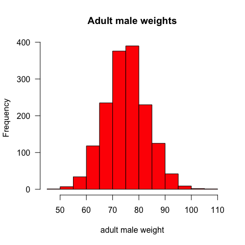
#Simulation of the weight of 1570 adult males normally distributed
data1=rnorm(1570,mean=75,sd=8)
hist(data1,main="Adult male weights",xlab="adult male weight",col="red",las=1)
Load example data
data = read.table("../Data/Simone/das.txt",header=T)
Visualize example data
attach(data) #command search() helps to verify what is/is not attached)
par(mfrow=c(2,2)) #to divide the plot window
plot(y)
boxplot(y)
hist(y,breaks=20)
y2=y
y2[52]=21.75 # to change the 52nd value for 21.75 instead of 2.175:
plot(y2)     #very good to spot mistakes, outliers

par(mfrow=c(1,1)) #back to one plot window
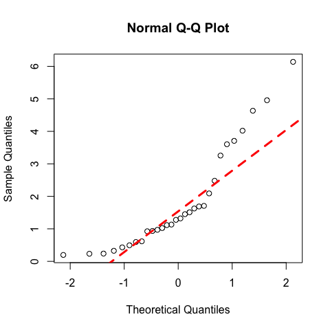
Visual Check for Normality: quantile-quantile plot
This one plots the ranked samples from our distribution against a similar number of ranked quantiles taken from a normal distribution. If our sample is normally distributed then the line will be straight. Exceptions from normality show up different sorts of non-linearity (e.g. S-shapes or banana shapes).
qqnorm(y)
qqline(y,lty=2,col=2,lwd=3)
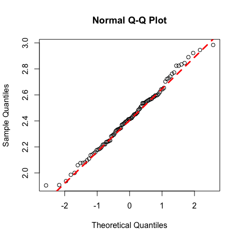
Normality test: the shapiro.test
shapiro.test(y) # p-value=0.753, these data are normally distributed
##
## 	Shapiro-Wilk normality test
##
## data:  y
## W = 0.9911, p-value = 0.753
detach(data)
As an example we will create a fake data log-normally distributed and verify the assumption of normality
x=exp(rnorm(30))  #rnorm without specification (normal distributed or not) picks data from the standard normal, mean = 0, sd = 1
plot(x)

boxplot(x)

hist(x,breaks=50)

qqnorm(x)
qqline(x,lty=2,col=2,lwd=3)
shapiro.test(x) #p-value=8.661e-07, not normally distributed
##
## 	Shapiro-Wilk normality test
##
## data:  x
## W = 0.8531, p-value = 0.0007207
Correlations tests
Correlation tests measure the relationship between variables. This relationship can goes from +1 to -1, where 0 means no relation. Some of the tests that we can use to estimate this relationship are the following:
-Pearson’s correlation is a parametric measure of the linear association between 2 numeric variables (PARAMETRIC TEST)
-Spearman’s rank correlation is a non-parametric measure of the monotonic association between 2 numeric variables (NON-PARAMETRIC TEST)
-Kendall’s rank correlation is another non-parametric measure of the associtaion, based on concordance or discordance of x-y pairs (NON-PARAMETRIC TEST)
attach(mtcars)
plot(hp,wt, main="scatterplot",las=1, xlab ="gross horse power", ylab="Weight (lb/1000)")

Compute the three correlation coefficients
cor(hp,wt,method="pearson")
## [1] 0.6587479
cor(hp,wt)#Pearson is the default method; the order of variables is not important
## [1] 0.6587479
cor(hp,wt,method="spearman")
## [1] 0.7746767
cor(hp,wt,method="kendal")
## [1] 0.6113081
`
Test the null hypothesis, that means that the correlation is 0 (there is no correlation)
cor.test(hp,wt,method="pearson") #Pearson correlation test
##
## 	Pearson's product-moment correlation
##
## data:  hp and wt
## t = 4.7957, df = 30, p-value = 4.146e-05
## alternative hypothesis: true correlation is not equal to 0
## 95 percent confidence interval:
##  0.4025113 0.8192573
## sample estimates:
##       cor
## 0.6587479
cor.test(hp,wt,method="spearman") #Spearmn is a non-parametric, thus it is not possible to get CIs. There is a error message because R cannot compute exact p values (the test is based on ranks, we have few cars with the same hp or wt).We can get rid off the warning letting R know that approximate values are fine
## Warning in cor.test.default(hp, wt, method = "spearman"): Cannot compute
## exact p-value with ties
##
## 	Spearman's rank correlation rho
##
## data:  hp and wt
## S = 1229.364, p-value = 1.954e-07
## alternative hypothesis: true rho is not equal to 0
## sample estimates:
##       rho
## 0.7746767
cor.test(hp,wt,method="spearman",exact=F)
##
## 	Spearman's rank correlation rho
##
## data:  hp and wt
## S = 1229.364, p-value = 1.954e-07
## alternative hypothesis: true rho is not equal to 0
## sample estimates:
##       rho
## 0.7746767
cor.test(hp,wt,method="kendal",exact=F) #same happens with Kendal correlation test
##
## 	Kendall's rank correlation tau
##
## data:  hp and wt
## z = 4.845, p-value = 1.266e-06
## alternative hypothesis: true tau is not equal to 0
## sample estimates:
##       tau
## 0.6113081
When we have non-parametric data and we do not know which correlation method to choose, as a rule of thumb, if the correlation looks non-linear, Kendall tau should be better than Spearman Rho.
Further handy functions for correlations
Plot all possible combinations with “pairs”
pairs(mtcars) # all possible pairwise plots

To make it simpler we select what we are interested
names(mtcars)
##  [1] "mpg"  "cyl"  "disp" "hp"   "drat" "wt"   "qsec" "vs"   "am"   "gear"
## [11] "carb" "fam"
pairs(mtcars[,c(1,4,6)]) # subsetting the categories we will use

Building a correlation matrix
#cor(mtcars)
cor(mtcars[,c(1,4,6)])
##            mpg         hp         wt
## mpg  1.0000000 -0.7761684 -0.8676594
## hp  -0.7761684  1.0000000  0.6587479
## wt  -0.8676594  0.6587479  1.0000000
detach(mtcars)
References
- Ruxton, G. D. (2006). The unequal variance t-test is an underused alternative to Student??????s t-test and the Mann-Whitney U test. Behavioral Ecology, 17, 688-690.
- Zimmerman, D. W. (2012). A note on consistency of non-parametric rank tests and related rank transformations. British Journal of Mathematical and Statistical Psychology, 65, 122-44.
- http://www.uni-kiel.de/psychologie/rexrepos/rerDescriptive.html