Disclaimer: All methods were presented by the us (the authors), who are not the package developers (apart from a few cases) and hence are not responsible for the accuracy, the errors or bugs in the functions. Please get in touch with the package maintainers if you have any problem.
Also, while we tried our best to introduce the functions, please make sure that you understand them: we may have used it wrongly!
Simulating spatially autocorrelated data in R using FReibier
We can simulate data sets using the function simData in FReibier (on github, not on CRAN). It offers simple, realistic or real environments, and 4 different ways to generate spatial autocorrelation (1. as autocorrelated error, 2. as missing variable, 3. as wrongly specified variable and 4. as mass effect).
Here, we shall use the missing-variable approach to see whether the latent variable approaches produce something akin to the missing variable.
The function simulates normal, Poisson or Bernoulli data, and a function to simulate the response can be provided. We shall use default settings.
Also different sizes of grids can be simulated.
First, we install the package from github:
library(devtools)
install_github("biometry/FReibier/FReibier")
Then we can read the help for \code{simData}:
library(FReibier, quietly = T)
`?`(simData)
Now we simulate a data set with binary response variable, a realistic landscape, SAC through omitted predictor, and a grid of 100 x 100 cells. For those approaches assuming normally distributed data, we use the same settings but a normal distribution:
simData("222", filename = "d222.100x100", gridsize = c(40, 40))  # binary
simData("212", filename = "d212.100x100", gridsize = c(40, 40))  # normal
This produces a netcdf-file, placed in the working directory, with all relevant data and the information about the data generation in it. We load it into R and have a look at the spatial autocorrelation in the model residuals.
d222full <- extract.ncdf("d222.100x100.nc")
d222full[[1]]  # meta-information
## $General_Information
## [1] "Gridsize = 40x40 cells; Random seed = 20151126; Number of predictors = 7; Block size for CV = 10x10 cells"
##
## $Landscape_predictors
## [1] "Realistic landscape: The 7 predictors are simulated unconditional Gaussian random fields from exponential covariance models with variance = 0.1,0.1,0.1,0.1,0.1,0.1,0.1 and scale = 0.1,0.1,0.1,0.1,0.1,0.1,0.1. These 7 predictors are rescaled to [-1,1]."
##
## $Response_distribution
## [1] "Bernoulli"
##
## $SAC_Scenario
## [1] "Omitted predictor."
##
## $Model_structure
## [1] "Model structure to use: y ~ x4 + x4^2 + x3*x4 + x3 + x2 + x5 + x6 + x7"
##
## $Response_coefficients
## [1] "0.2 + 4.5 * x1+1.2 * x4+-1.2 * x4^2+-1.1 * x3*x4+0.9 * x3"
d222 <- d222full[[2]]  # extract only the data
d212 <- extract.ncdf("d222.100x100.nc")[[2]]
library(lattice)
levelplot(y ~ Lon + Lat, data = d222)  # what the response looks like
# fit the model:
form <- as.formula("y ~ x4 + I(x4^2) + x3*x4 + x3 + x2 + x5 + x6 + x7")  # extracts formula from simulated data
summary(fglm <- glm(form, data = d222, family = binomial))
##
## Call:
## glm(formula = form, family = binomial, data = d222)
##
## Deviance Residuals:
##     Min       1Q   Median       3Q      Max
## -1.5880  -1.2257   0.8924   1.0741   1.7037
##
## Coefficients:
##             Estimate Std. Error z value Pr(>|z|)
## (Intercept)  0.19989    0.06750   2.961 0.003062 **
## x4           0.99258    0.19883   4.992 5.98e-07 ***
## I(x4^2)     -0.77567    0.51974  -1.492 0.135592
## x3           0.56449    0.16757   3.369 0.000756 ***
## x2          -0.39300    0.16057  -2.447 0.014385 *
## x5           0.41155    0.18327   2.246 0.024727 *
## x6          -0.03506    0.16666  -0.210 0.833388
## x7          -0.18379    0.16289  -1.128 0.259194
## x4:x3       -0.96851    0.67373  -1.438 0.150569
## ---
## Signif. codes:  0 '***' 0.001 '**' 0.01 '*' 0.05 '.' 0.1 ' ' 1
##
## (Dispersion parameter for binomial family taken to be 1)
##
##     Null deviance: 2207.5  on 1599  degrees of freedom
## Residual deviance: 2149.1  on 1591  degrees of freedom
## AIC: 2167.1
##
## Number of Fisher Scoring iterations: 4
summary(fglmGaus <- glm(form, data = d212, family = gaussian))
##
## Call:
## glm(formula = form, family = gaussian, data = d212)
##
## Deviance Residuals:
##     Min       1Q   Median       3Q      Max
## -0.7239  -0.5279   0.3275   0.4399   0.7794
##
## Coefficients:
##              Estimate Std. Error t value Pr(>|t|)
## (Intercept)  0.548229   0.016201  33.839  < 2e-16 ***
## x4           0.239328   0.047171   5.074 4.36e-07 ***
## I(x4^2)     -0.176980   0.120508  -1.469 0.142136
## x3           0.135685   0.039872   3.403 0.000683 ***
## x2          -0.093630   0.038346  -2.442 0.014726 *
## x5           0.099769   0.043972   2.269 0.023405 *
## x6          -0.008485   0.039930  -0.212 0.831752
## x7          -0.044154   0.039166  -1.127 0.259765
## x4:x3       -0.233504   0.159081  -1.468 0.142347
## ---
## Signif. codes:  0 '***' 0.001 '**' 0.01 '*' 0.05 '.' 0.1 ' ' 1
##
## (Dispersion parameter for gaussian family taken to be 0.2407715)
##
##     Null deviance: 397.36  on 1599  degrees of freedom
## Residual deviance: 383.07  on 1591  degrees of freedom
## AIC: 2273.3
##
## Number of Fisher Scoring iterations: 2
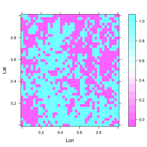
Figure: A plot of the response in space.
The region has coordinates between 0 and 1 in each direction, for simplicity.
Diagnostics and Timing
(also explain correlog, possibly Moran’s I, system.time, residual maps;)
Correlogram
Now, for the correlogram (which is one way of visualising spatial autocorrelation), there are different options. We do a quick speed-test, as we will use this function for every method and should thus choose a fast one. Note that each computation takes quite a bit of time, as the data set is relatively large; so we take only the first 1000 data points for the trials.
# library(pgirmess) system.time(correlPGIR <-
# pgirmess::correlog(d222[1:1000, 2:3],
# z=residuals(fglm)[1:1000]))
library(ncf)
system.time(correlNCF <- ncf::correlog(d222[1:1000, 2], d222[1:1000,
    3], z = residuals(fglm)[1:1000], increment = 0.025, resamp = 1))
##    user  system elapsed
##   1.805   0.091   1.951
# library(spind) system.time(correlSPIND <-
# spind::acfft(round(d222[1:1000, 2:3]*1000),
# residuals(fglm)[1:1000], lim1=0, lim2=500)) # needs integer
# coordinates
And the winner is: correlog in ncf (by an order of magnitude!). See also here for other packages computing correlograms.
For the full 10000 data points this takes over 3 minutes!
We now show the reduction in spatial autocorrelation from raw data to GLM residuals:
correlNCFraw <- ncf::correlog(d222[, 2], d222[, 3], z = d222$y,
    increment = 0.025, resamp = 1)
correlNCF <- ncf::correlog(d222[, 2], d222[, 3], z = residuals(fglm),
    increment = 0.025, resamp = 1)
correlFglmGaus <- ncf::correlog(d222[, 2], d222[, 3], z = residuals(fglmGaus),
    increment = 0.025, resamp = 1)
plot(correlNCFraw$mean.of.class, correlNCFraw$correlation, type = "o",
    pch = 16, xlim = c(0, 0.5), ylim = c(-0.1, 0.2), las = 1,
    lwd = 2, xlab = "distance", ylab = "Moran's I")  # show for half the size of the region
abline(h = 0, col = "grey")
lines(correlNCF$mean.of.class, correlNCF$correlation, lwd = 2,
    col = "green")
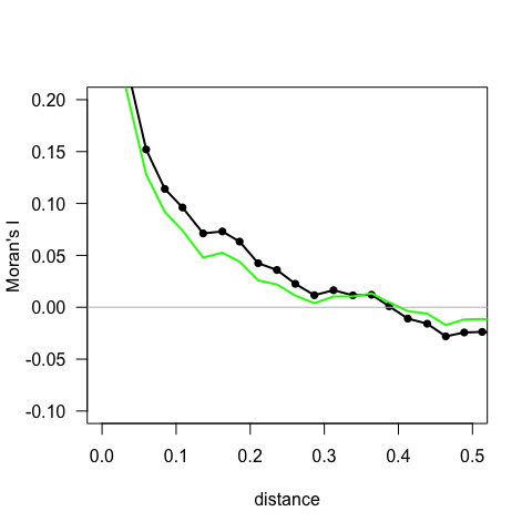
Figure: A correlogram, representing the correlation of the spatially shifted data set as a function of the distance shifted. Black dots and line are raw y-data, green line is based on GLM-residuals.
You can choose finer or coarser increments, of course. Note that large distances have few data points behind them (as you can see when investigating the correlogNCF-object using str), that’s why we cut off the values for distances larger than 0.5.
What we see is that there is some (mild) spatial autocorrelation until a distance of 0.2 or so, when it starts levelling off. Using the option resampling=100, you can also test each distance bin for significance. NOTE that this then takes 100 times as long!
(Semi-)variogram
The semi-variogram is the more common form to visualise spatial autocorrelation for those used to GIS and kriging, rather than spatial regression models.
Just like the correlogram, there are several implementations in R (adespatial, automap, ctmm, fields, geoR/geoRglm, georob, gstat, nlme, RandomFields, rtop, sm, spatial, SpatialExtremes, to name only a few).
library(fields)
VG <- vgram(loc = d222[, 1:2], y = residuals(fglm), N = 20, dmax = 1)
plot(VG, las = 1)
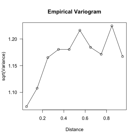
Figure: Variogram of model residuals.
The distance where the semi-variogram levels off (around 0.3 or so) should be the same as where the correlogram hits 0, i.e. the range of spatial autocorrelation. This is more difficult to see here.
Global Moran’s I
One can compute Moran’s I for the entire data, based on the neighbourhood (or distance) matrix. Again, plenty of implementations exist, differing in the way the neighbourhood is set up. We use one of the fastest:
library(ape)
##
## Attaching package: 'ape'
## The following object is masked from 'package:ncf':
##
##     mantel.test
## The following objects are masked from 'package:raster':
##
##     rotate, zoom
Dists <- as.matrix(dist(d222[, 1:2]))
diag(Dists) <- 0  #distances on diagonal must be set to 0
Moran.I(residuals(fglm), Dists)
## $observed
## [1] -0.01890117
##
## $expected
## [1] -0.0006253909
##
## $sd
## [1] 0.000507135
##
## $p.value
## [1] 2.180356e-284
This indicates that the model residuals of the GLM still carry a significant amount of spatial autocorrelation.
Map of residuals
Since the data are spatial, we can plot a map. A map of residuals typically gives us a feeling for the degree of clumping, and may also indicate which additional variable may be useful in the model.
The simplest way to map residuals we already encountered:
levelplot(residuals(fglm) ~ Lon + Lat, data = d222)
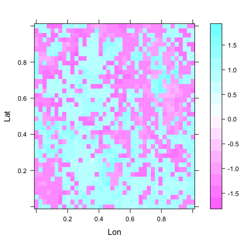
Figure: Map of model residuals. This should, in an ideal world, show no pattern at all, neither gradients nor clustering. In this case, the clustering is very similar as in the raw data, although differently arranged. Clearly the GLM does not remove the spatial autocorrelation to any noticeable extent (see previous figures).