Explorative data analysis has the goal to explore and describe the patterns in your data, without any particular hypothesis.
Good introductions on this topic
-
See further discussion in the Essential Statistics lecture notes, chapter on descriptive statistics as well as appendix on graphics and summary statistics
-
For more details about plotting, please visit: http://biometry.github.io/APES/R/R40-plottingInR.html
Some examples in R
Exploring categorical data
Summary statistics
Some piece of information that gives a quick and simple description of the data.
attach(mtcars)
head(mtcars)
##                    mpg cyl disp  hp drat    wt  qsec vs am gear carb
## Mazda RX4         21.0   6  160 110 3.90 2.620 16.46  0  1    4    4
## Mazda RX4 Wag     21.0   6  160 110 3.90 2.875 17.02  0  1    4    4
## Datsun 710        22.8   4  108  93 3.85 2.320 18.61  1  1    4    1
## Hornet 4 Drive    21.4   6  258 110 3.08 3.215 19.44  1  0    3    1
## Hornet Sportabout 18.7   8  360 175 3.15 3.440 17.02  0  0    3    2
## Valiant           18.1   6  225 105 2.76 3.460 20.22  1  0    3    1
fam=mtcars$fam=factor(mtcars$am, levels=c(0,1), labels=c("automatic","manual"))
#we substract the variable Transmission (0 = automatic, 1 = manual) with "$" from the dataset
head(mtcars)
##                    mpg cyl disp  hp drat    wt  qsec vs am gear carb
## Mazda RX4         21.0   6  160 110 3.90 2.620 16.46  0  1    4    4
## Mazda RX4 Wag     21.0   6  160 110 3.90 2.875 17.02  0  1    4    4
## Datsun 710        22.8   4  108  93 3.85 2.320 18.61  1  1    4    1
## Hornet 4 Drive    21.4   6  258 110 3.08 3.215 19.44  1  0    3    1
## Hornet Sportabout 18.7   8  360 175 3.15 3.440 17.02  0  0    3    2
## Valiant           18.1   6  225 105 2.76 3.460 20.22  1  0    3    1
##                         fam
## Mazda RX4            manual
## Mazda RX4 Wag        manual
## Datsun 710           manual
## Hornet 4 Drive    automatic
## Hornet Sportabout automatic
## Valiant           automatic
Frequency table of the Transmission variable
table(fam)
## fam
## automatic    manual
##        19        13
count=table(fam)
count
## fam
## automatic    manual
##        19        13
% frequencies calculation
percent=table(fam)/length(fam)
percent
## fam
## automatic    manual
##   0.59375   0.40625
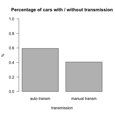
Bar charts
Bar charts are appropiate to summarize categorical variables distributions
barplot(percent, main="Percentage of cars with / without transmission", xlab="transmission", ylab="%", las=1, ylim=c(0,1), names.arg=c("auto transm", "manual transm") )
Exploring continous / categorical data
Summary statistics
For a numerical variable, like “mpg”
mean(mpg)
## [1] 20.09062
summary(mpg)
##    Min. 1st Qu.  Median    Mean 3rd Qu.    Max.
##   10.40   15.42   19.20   20.09   22.80   33.90
sd(mpg) #standard deviation
## [1] 6.026948
var(mpg) #variance
## [1] 36.3241
sqrt(var(mpg)) # = to sd
## [1] 6.026948
sd(mpg)^2 # = to variance
## [1] 36.3241
max(mpg)
## [1] 33.9
tapply(mpg,fam,mean)
## automatic    manual
##  17.14737  24.39231
tapply(mpg,list(fam,gear),mean)
##                  3      4     5
## automatic 16.10667 21.050    NA
## manual          NA 26.275 21.38
Boxplot
Boxplots are appropiate to summarize numerical variables distributions
summary(mpg)
##    Min. 1st Qu.  Median    Mean 3rd Qu.    Max.
##   10.40   15.42   19.20   20.09   22.80   33.90
quantile(mpg)
##     0%    25%    50%    75%   100%
## 10.400 15.425 19.200 22.800 33.900
quantile(mpg,probs=c(0,0.20,0.40,0.60,0.80,1))
##    0%   20%   40%   60%   80%  100%
## 10.40 15.20 17.92 21.00 24.08 33.90
boxplot(mpg~fam, main="mpg by transmission")

Histograms
Histograms are appropiate to summarize numerical variables distributions
hist(mpg)

Stem and Leaf Plots
Stem and Leaf plots are appropiate to summarize numerical variables distributions (low sample size)
stem(mpg)
##
##   The decimal point is at the |
##
##   10 | 44
##   12 | 3
##   14 | 3702258
##   16 | 438
##   18 | 17227
##   20 | 00445
##   22 | 88
##   24 | 4
##   26 | 03
##   28 |
##   30 | 44
##   32 | 49
?stem for more info
There are 2 obs 10.4
There is one obs 32.4 and one 32.9
Scatterplots
Scatterplots are appropiate to summarize the relation between two numerical variables
Relation ship between horsepower hp and consumption mpg
plot(mpg~hp) # y~x

plot(hp, mpg) # x,y

plot(hp, mpg,xlab = "Gross horsepower", ylab="Miles/(US) gallon", las=1, col="red", xlim=c(0,400), cex =2 )
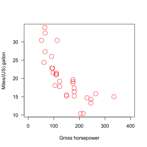
#cex (plotting characters size times 2)